2021.10.15 - [Study/Deep Learning] - TensorFlow 2.0과 Softmax Regression을 이용한 MNIST 숫자분류기 구현
TensorFlow 2.0과 Softmax Regression을 이용한 MNIST 숫자분류기 구현
<가설 정의> 1. MNIST 데이터를 불러와 학습하기 적합한 형태로 변형 # -*- coding: utf-8 -*- import tensorflow as tf # MNIST 데이터를 다운로드 (x_train, y_train), (x_test, y_test) = tf.keras.datasets.mn..
these-dayss.tistory.com
이전 글을 참고하면 이해가 잘 갈 것이다.
# -*- coding: utf-8 -*-
# 텐서플로우를 이용한 ANN(Artificial Neural Networks) 구현 - Keras API를 이용한 구현

import tensorflow as tf

# MNIST 데이터를 다운로드
(x_train, y_train), (x_test, y_test) = tf.keras.datasets.mnist.load_data()
# 이미지들을 float32 데이터 타입으로 변경
x_train, x_test = x_train.astype('float32'), x_test.astype('float32')
# 28*28 형태의 이미지를 784차원으로 flattening 함
x_train, x_test = x_train.reshape([-1, 784]), x_test.reshape([-1, 784])
# [0, 255] 사이의 값을 [0, 1]사이의 값으로 Normalize 함
x_train, x_test = x_train / 255., x_test / 255.
# 레이블 데이터에 one-hot encoding을 적용
y_train, y_test = tf.one_hot(y_train, depth=10), tf.one_hot(y_test, depth=10)

# 학습을 위한 설정값들을 정의
learning_rate = 0.001
num_epochs = 30     # 학습횟수
batch_size = 256    # 배치개수
display_step = 1    # 손실함수 출력 주기
input_size = 784    # 28 * 28
hidden1_size = 256
hidden2_size = 256
output_size = 10

# tf.data API를 이용해서 데이터를 섞고 batch 형태로 가져옴
train_data = tf.data.Dataset.from_tensor_slices((x_train, y_train))
train_data = train_data.shuffle(60000).batch(batch_size) # 한번 epoch가 끝날 때마다 셔플(섞어줌)

# 초기 W값과 b 값을 초기화
def random_normal_intializer_with_stddev_1():
  return tf.keras.initializers.RandomNormal(mean=0.0, stddev=1.0, seed=None)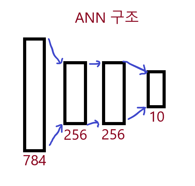
# tf.keras.Model을 이용해서 ANN 모델을 정의
class ANN(tf.keras.Model):
  def __init__(self):
    super(ANN, self).__init__()
    self.hidden_layer_1 = tf.keras.layers.Dense(hidden1_size,
                                                activation='relu',
                                                kernel_initializer=random_normal_intializer_with_stddev_1(),
                                                bias_initializer=random_normal_intializer_with_stddev_1())
    self.hidden_layer_2 = tf.keras.layers.Dense(hidden2_size,
                                                activation='relu',
                                                kernel_initializer=random_normal_intializer_with_stddev_1(),
                                                bias_initializer=random_normal_intializer_with_stddev_1())
    self.output_layer = tf.keras.layers.Dense(output_size,
                                              activation=None,
                                              kernel_initializer=random_normal_intializer_with_stddev_1(),
                                              bias_initializer=random_normal_intializer_with_stddev_1())

  def call(self, x):
    H1_output = self.hidden_layer_1(x)
    H2_output = self.hidden_layer_2(H1_output)
    logits = self.output_layer(H2_output)

    return logits
# cross-entropy 손실 함수를 정의
@tf.function
def cross_entropy_loss(logits, y):
  return tf.reduce_mean(tf.nn.softmax_cross_entropy_with_logits(logits=logits, labels=y))

# 최적화를 위한 Adam 옵티마이저를 정의, 기본 옵티마이저를 업그레이드 한 것. 미분값이 0인 곳도 넘어감
optimizer = tf.optimizers.Adam(learning_rate)

# 최적화를 위한 function을 정의
@tf.function
def train_step(model, x, y):  #한 번의 Gradient Descent 수행
  with tf.GradientTape() as tape:
    y_pred = model(x)
    loss = cross_entropy_loss(y_pred, y)
  gradients = tape.gradient(loss, model.trainable_variables)
  optimizer.apply_gradients(zip(gradients, model.trainable_variables))

# 모델의 정확도를 출력하는 함수를 정의
@tf.function
def compute_accuracy(y_pred, y):
  correct_prediction = tf.equal(tf.argmax(y_pred,1), tf.argmax(y,1))
  accuracy = tf.reduce_mean(tf.cast(correct_prediction, tf.float32))

  return accuracy
# ANN 모델을 선언
ANN_model = ANN()

# 지정된 횟수만큼 최적화를 수행
for epoch in range(num_epochs):
  average_loss = 0.
  total_batch = int(x_train.shape[0] / batch_size)
  # 모든 배치들에 대해서 최적화를 수행
  for batch_x, batch_y in train_data:
    # 옵티마이저를 실행해서 파라마터들을 업데이트
    _, current_loss = train_step(ANN_model, batch_x, batch_y), cross_entropy_loss(ANN_model(batch_x), batch_y)
    # 평균 손실을 측정
    average_loss += current_loss / total_batch
  # 지정된 epoch마다 학습결과를 출력
  if epoch % display_step == 0:
    print("반복(Epoch): %d, 손실 함수(Loss): %f" % ((epoch+1), average_loss))

# 테스트 데이터를 이용해서 학습된 모델이 얼마나 정확한지 정확도를 출력
print("정확도(Accuracy): %f" % compute_accuracy(ANN_model(x_test), y_test)) # 정확도: 약 94%
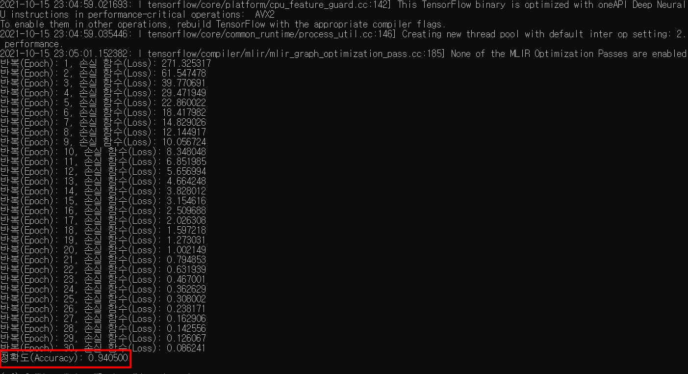
epoch 횟수 별로 손실함수 값이 어떻게 변화하는지 알 수 있다.
(한 번의 epoch는 인공 신경망에서 전체 데이터 셋에 대해 forward pass/backward pass 과정을 거친 것을 말함. 즉, 전체 데이터 셋에 대해 한 번 학습을 완료한 상태)
epoch가 반복되면서 손실함수 값이 점진적으로 감소하는 것을 알 수 있고
30번 모두 끝난 후의 모델의 학습 정확도를 계산해보면 약 94%임을 알 수 있다.
'Study > Deep Learning' 카테고리의 다른 글
| CNN 의 등장 (0) | 2021.10.16 |
|---|---|
| 오토인코더 Autoencoder (0) | 2021.10.15 |
| 다층 퍼셉트론 MLP (0) | 2021.10.15 |
| TensorFlow 2.0과 Softmax Regression을 이용한 MNIST 숫자분류기 구현 (0) | 2021.10.15 |
| TensorFlow 2.0을 이용한 선형 회귀(Linear Regression) 알고리즘 구현 (0) | 2021.10.15 |