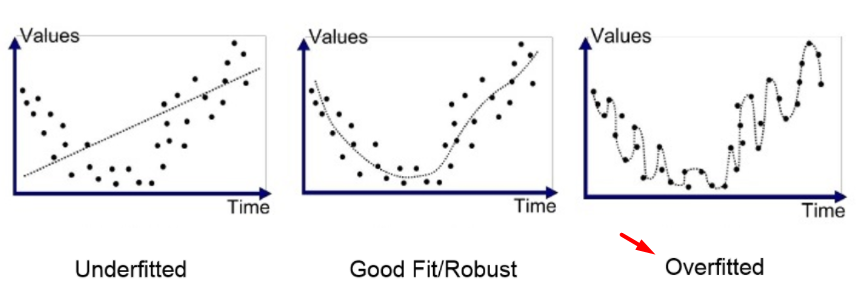
<가설 정의>
1. MNIST 데이터를 불러와 학습하기 적합한 형태로 변형
# -*- coding: utf-8 -*-

import tensorflow as tf

# MNIST 데이터를 다운로드
(x_train, y_train), (x_test, y_test) = tf.keras.datasets.mnist.load_data()
load_data() 호출 시 MNIST 데이터를 numpy (int)array 형태로 반환해줌
x_train, y_train에는 약 60000개의 트레이닝 데이터, x_test, y_test에는 약 10000개의 테스트 데이터가 있음
# 이미지들을 float32 데이터 타입으로 변경
x_train, x_test = x_train.astype('float32'), x_test.astype('float32')
# 28*28 형태의 이미지를 784차원으로 flattening 함
x_train, x_test = x_train.reshape([-1, 784]), x_test.reshape([-1, 784])
# [0, 255] 사이의 값을 [0, 1]사이의 값으로 Normalize 함
x_train, x_test = x_train / 255., x_test / 255.
astype : 데이터 형변환
reshape(-1,~) : 여기서 -1은 매직넘버. 앞 차원에 알아서 맞춰줌. 기본 옵션이라고 생각
flattening : 2차원 데이터를 한 픽셀씩 펼쳐서 1차원 데이터로 변경하는 것. 28*28 -> 784
MNIST 데이터는 픽셀 하나당 0-255까지의 숫자값을 가지므로 ,이를 255로 나누면 0-1 사이로 normalize 됨
# 레이블 데이터에 one-hot encoding을 적용
y_train, y_test = tf.one_hot(y_train, depth=10), tf.one_hot(y_test, depth=10)
정답 데이터가 int 형이므로 one-hot encoding 을 적용해준다.
( 1 → 1000000000, 2 → 0100000000, 3 → 0010000000 이런 형식)
2. 전체 데이터를 원하는 mini-batch 개수만큼 묶어줌
# tf.data API를 이용해서 데이터를 섞고 batch 형태로 가져옴
train_data = tf.data.Dataset.from_tensor_slices((x_train, y_train))
train_data = train_data.repeat().shuffle(60000).batch(100)
train_data_iter = iter(train_data)
tf.data.Dataset : api. 미니배치 단위로 묶는 과정을 손쉽게 할 수 있도록 함
iter : iterator. 100개씩의 미니배치를 순차적으로 가리키게 됨
3. 소프트맥스 회귀 모델 정의
# tf.keras.Model을 이용해서 Softmax Regression 모델을 정의
class SoftmaxRegression(tf.keras.Model):
  def __init__(self):
    super(SoftmaxRegression, self).__init__()
    self.softmax_layer = tf.keras.layers.Dense(10,
                                               activation=None,
                                               kernel_initializer='zeros',
                                               bias_initializer='zeros')

  def call(self, x):
    logits = self.softmax_layer(x)

    return tf.nn.softmax(logits)
tf.keras.Model : 상속받는 클래스
tf.keras.layers.Dense : Wx+b를 추상화 해놓은 api (input을 넣었을 때 output으로 바꿔주는 중간 다리)
→ 10 = units. 출력 값의 크기, activation = 활성화 함수, kernel_initializer = 가중치(W) 초기화 함수, bias_initializer = 편향(b) 초기화 함수
call : 클래스 호출 시 동작하는 함수
logits : softmax(Wx+b)가 적용된 10 dimension의 값이 담겨있음
<손실함수 정의>
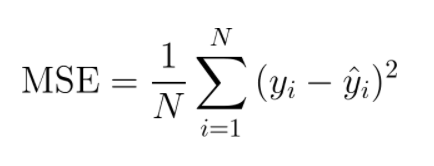
# cross-entropy 손실 함수를 정의
@tf.function
def cross_entropy_loss(y_pred, y):
  return tf.reduce_mean(-tf.reduce_sum(y * tf.math.log(y_pred), axis=[1]))
  #return tf.reduce_mean(tf.nn.softmax_cross_entropy_with_logits(logits=logtis, labels=y)) # tf.nn.softmax_cross_entropy_with_logits API를 이용한 구현
<최적화>
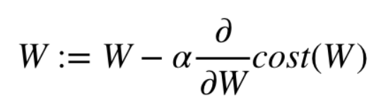
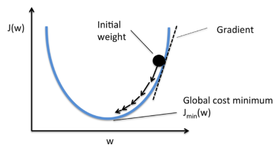
# 최적화를 위한 그라디언트 디센트 옵티마이저를 정의
optimizer = tf.optimizers.SGD(0.5)

# 최적화를 위한 function을 정의
@tf.function
def train_step(model, x, y):
  with tf.GradientTape() as tape:
    y_pred = model(x)
    loss = cross_entropy_loss(y_pred, y)
  gradients = tape.gradient(loss, model.trainable_variables)
  optimizer.apply_gradients(zip(gradients, model.trainable_variables))
SGD : 옵티마이저 종류 중 하나
0.5 : learning rate
# 모델의 정확도를 출력하는 함수를 정의
@tf.function
def compute_accuracy(y_pred, y):  #모델이 예측한 값, 정답값
  correct_prediction = tf.equal(tf.argmax(y_pred,1), tf.argmax(y,1))  #일치 개수 반환
  accuracy = tf.reduce_mean(tf.cast(correct_prediction, tf.float32))  #0~1 사이의 정확도 반환

  return accuracy
argmax : 최대값을 갖는 성분의 인덱스를 반환
y_pred는 softmax 함수 결과 값이 들어있다. [0.01, 0.4, 0.7, 0.04, 0.2, 0.082, 0.03, 0.002, 0.3, 0.06]
하지만 정답값 y에는 [0, 0, 1, 0, 0, 0, 0, 0, 0, 0] 과 같은 형식으로 들어있다.
따라서 y_pred에 argmax 함수를 취하여 최대값을 갖는 성분의 인덱스를 반환하여 비교시키는 작업이 필요하다
# SoftmaxRegression 모델을 선언
SoftmaxRegression_model = SoftmaxRegression()
# 1000번 반복을 수행하면서 파라미터 최적화를 수행
for i in range(1000):
batch_xs, batch_ys = next(train_data_iter) #100개씩의 mini-batch 데이터가 반환
train_step(SoftmaxRegression_model, batch_xs, batch_ys)
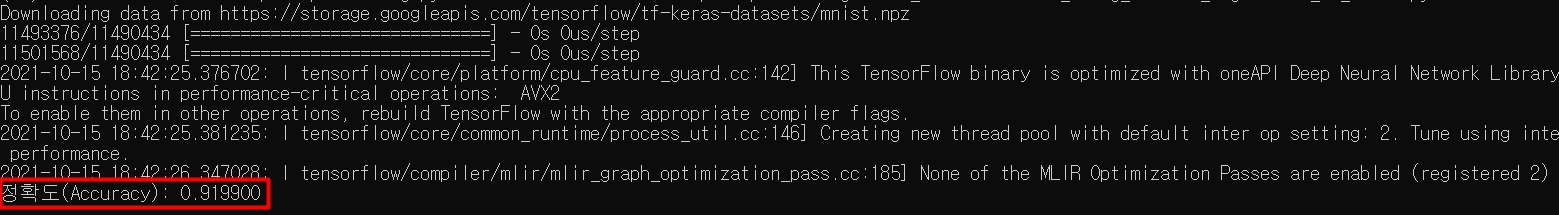
# 학습이 끝나면 학습된 모델의 정확도를 출력
print("정확도(Accuracy): %f" % compute_accuracy(SoftmaxRegression_model(x_test), y_test)) # 정확도 : 약 91%batch_xs : (100, 784) MNIST 데이터
batch_ys : 100 dimension의 원-핫 인코딩된 데이터
'Study > Deep Learning' 카테고리의 다른 글
| TensorFlow 2.0과 ANN을 이용한 MNIST 숫자분류기 구현 (0) | 2021.10.15 |
|---|---|
| 다층 퍼셉트론 MLP (0) | 2021.10.15 |
| TensorFlow 2.0을 이용한 선형 회귀(Linear Regression) 알고리즘 구현 (0) | 2021.10.15 |
| TensorFlow (0) | 2021.10.15 |
| 다양한 Computer Vision 문제 영역 (0) | 2021.10.14 |